Causal Probes

This project was selected from submissions on our Technical AI Safety Project sprint (Dec 2025). Participants worked on these projects for 1 week.

Problem Statement

We aim to develop a measure of a probe’s causalness and thus state, with high confidence, whether a probe is causal.

Hypothesis

By applying carefully designed causal interventions to the probe’s input, we can observe highly contrasting behaviors between causal and non-causal probes, thereby enabling causal verification.

Setup

We focus on probes over the Othello GPT model because game-based models have a visual component that is easier to verify and observe¹. The Othello GPT, given an input sequence of steps, computes the probability of all squares for the next step. For each square, there are three states: blank, black, and white, and a well-trained model can state with high confidence which state each square will occupy next.

We reuse the probes provided in² and introduce additional probes (self-trained and random tensors) to evaluate their outputs in the planned experiment.

Experiments

Given a well-trained Othello GPT, access to its residual streams (for each attention layer), and a probe, we aim to design an experiment to assess how a probe’s behavior changes under specific interventions. We use the following process per intervention,

1. Explain the what and the why behind an intervention.

2. State an intervention exactly (modification to input)

3. State expected output (how do we expect probabilities of squares to change) and make a causal claim for the probe.

def function(trained_gpt_residual_streams, probe, causal_intervention_func) -> boolean

The above function definition covers the initial thought process. We, however, note that causality, by itself, is not a Boolean variable; that is, it’s not always apparent whether a conclusion is causal even under specific observations. Thus, we prefer a per-intervention score-based metric, which provides a relative causal measure. We argue that relative causality adds substantial value by enabling probe selection through comparisons and by allowing multiple interventions (e.g., comparing multiple booleans is more difficult than simply reporting per-intervention scores and allowing the user to choose the appropriate investigation based on some weighted score).

def function(trained_gpt_residual_streams, probe, causal_intervention_func) -> float

The evolved function describes our updated thought process, and we will dedicate two sections to each experiment: first, to metric design, and second, to interventions.

Experiment #1

Translating predictive power to causality

What/Why? We expect well-trained models to be fitted to the distribution of their training set and thus to be highly opinionated and sensitive when we change an input from a known (in-distribution) sample to an out-of-distribution sample.

Intervention: Add a constant bias to the residual streams. Bias is computed as follows.

And we can have multiple scales of bias: a scale of zero implies no bias, whereas any non-zero scale yields non-zero bias that is directly proportional to the scale magnitude.

The idea is that we significantly shift the current residual stream in a measured, biased way by removing some learned capacity from it. Random vectors will not carry any semantic meaning, so we cannot simply expect to remove random values.

Metric Design: We expect that causal models will change predicted squares’ probabilities much more quickly than non-causal models by nature of their being more opinionated. Thus, we develop a metric to quantify the approximation that computes how quickly the scale probability for a specific board’s decision changes over the scales.

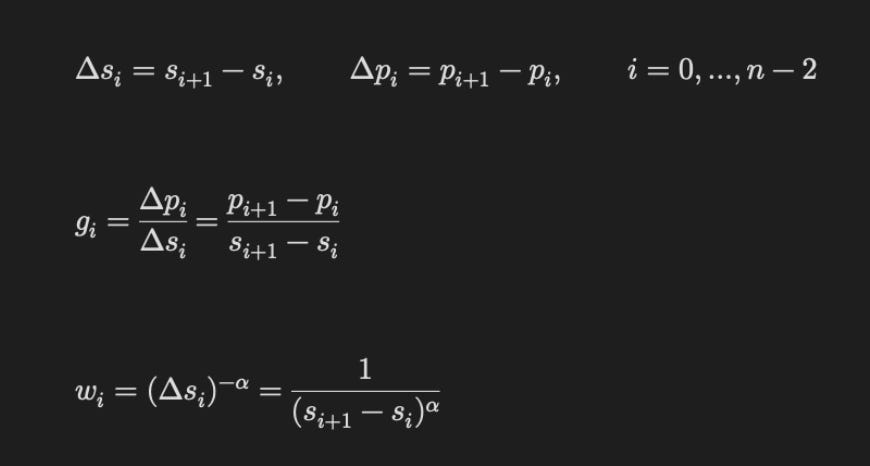
It’s represented as follows (we use the RMS score) and alpha = 2. Here, the Δpᵢ

\(\Delta p_i\)

means the change in probabilities over consecutive scales. And Δsᵢ shows how different consecutive scales are. gᵢ represents the change in the probability over the scales. We then convert these gradients into the gradient flow metric (RMS), using a specific weighting scheme that gives greater weight to faster changes over smaller-scale differences (based on how wᵢ is computed).

Table 1: Here, we represent the experiments from the causality discovery for probes. We observe that with a larger scale of forced bias, the high-quality probes (first two) quickly shift their decision to a different one. In contrast, the lowest-quality probe (random) barely shifts, and the moderately well-trained probe (slowly moves its decision away).

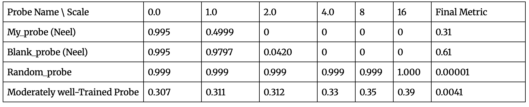
Note that we train the moderately trained probe on over 7500 samples (and the validation accuracy never exceeds 75%, so we expect the probe to exhibit weakly held opinions).

Here, the horizontal axis represents the scale of distortion of the probe’s decision. A larger scale indicates a higher bias. As expected, better-performing probes yield a higher final metric. Interestingly, the blank probe has a higher predictive probability, which we suggest is because it requires only one decision: whether any player covers the probe. But my_probe must make three decisions: whether it is the probe for either player, or whether it remains blank, thereby making its predictive power more distributed. Also, such a score helps narrate how far off my trained probe is from a high-quality probe. This is also evident from looking at the moderately trained probes’ probability scores in the first place.

Issue with Experiment #1

Experiment #1 appears sound; however, a fatal flaw in its hypothesis is that we could observe all probes with low train/validation losses, thereby adopting a more opinionated stance. But we note that even with a low loss value, causality can be missing in the following cases,

1. The input contains future data, which allows low loss via future leakage. Since we only feed past steps, we cannot have future information about the data (ideally, this is not a risk).

2. The input/setup contains a risk variable that encodes future information by virtue of its bias. For example, if we train only on games in which black always wins, the model may achieve a very low loss but also learn representations that simply predict moves for black (since the outcome is constant across all games).

   1. Note that similar risks can arise from duplicated training samples, from using games from a particular strategy (where all openings are identical), and from similar data biases.

We note that risk #2 is more likely, given that risk #1 is negated by feeding only explicitly past content to the base model and probes.

Suggested Future Experiment #2 (not complete)

What/Why? We could examine the input data and design a metric to determine whether a probe is misleadingly causal; however, we may have access to a probe but no access to training data for various reasons (e.g., privacy/copyright). Thus, we aim to understand the probe’s bias without accounting for any artifacts beyond access to the probe’s inference engine.

Interventions: To avoid biased probes being considered causal, we have two options: maintain a gold-standard set of samples and ensure low validation loss. But we may not always be able to develop such sets, and it’s costly to keep them. Instead, we could borrow ideas from red-teaming. For example, we could,

1. Use same-label consistency checks: For the same label (high probability on some square), do we get the exact predictions? If we do, it implies that the model is based on outcomes rather than shortcuts. However, this test can fail when the data in the validation set is too biased.

2. Instead, we will adopt a directional approach, focus on the PCA of activations, and determine whether, for a given probe, we can map how it behaves as a function of the activation direction. There is a comprehensive list of options that may occur here; we summarize them later in a more subjective manner.

Metric: We aim to provide a list of outputs to enable the user to select the principal components and the probe output. We can then attach a simple decision tree at the end to interpret the result. Given that probe development is costly (in terms of training) and that there are limited examples for building a decision tree, we instead provide a qualitative understanding and outline a blueprint for the decision tree.

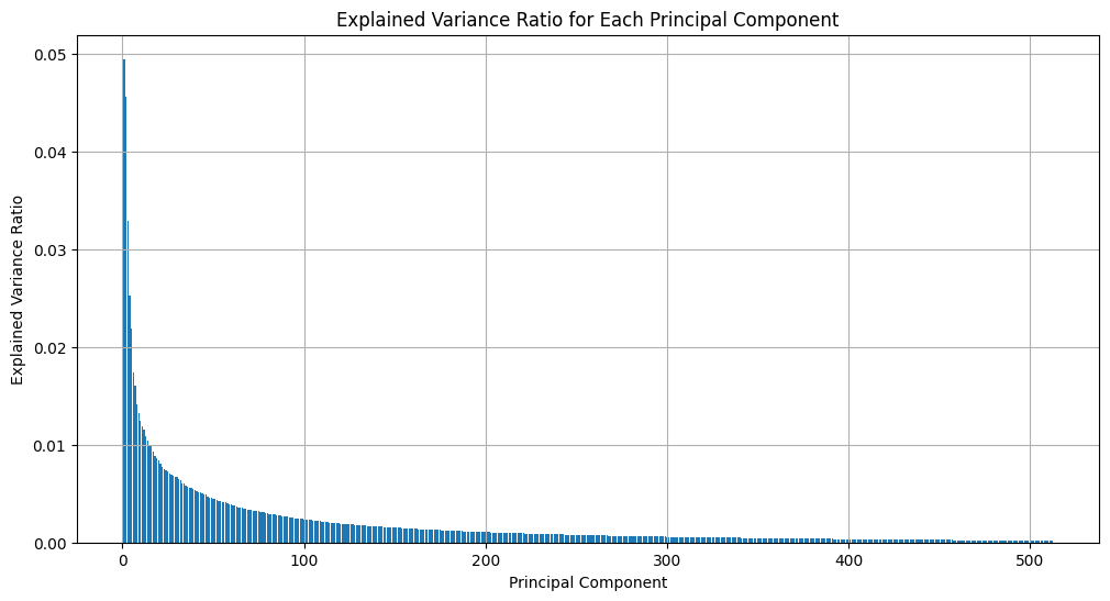
Results: We present the probabilistic outputs of the principal components (PCs) based on the current probe, along with their subsequent interpretations, below.

PCA from current activations showing variance distribution over the various principal components. We expect causality to show up distinctly based on how well the probes handle the various components of the activations.

1. https://www.alignmentforum.org/posts/nmxzr2zsjNtjaHh7x/actually-othello-gpt-has-a-linear-emergent-world#How_do_models_represent_features_

2. https://www.alignmentforum.org/posts/nmxzr2zsjNtjaHh7x/actually-othello-gpt-has-a-linear-emergent-world#How_do_models_represent_features_